TLS description of optical absorption
In this notebook we present a two level system (TLS) based description of optical absorption. We discuss the equation of motion of the system (EQM) in the rotating frame (RF) and we derive the Bloch vector representation of the model.
The Hamiltonian of the system is written as
The interaction of the optical pump with the system is described by an Hamiltonian \(H^I\) that has only non-diagonal non vanishing matrix elements.
The equation of motion (EQM) of the density matrix (DM) are expressed by the Liouville equation
It is convenient to describe the system in terms of polarization and of the inversion variables defined as
Interaction Hamiltonian and rotating wave approximation (RWA)
We consider an interaction between the system and the optical pump described by a dipole interaction, that is
The RWA can be used if we are interested in probing the system with energy of the pump not very different from the energy gap of the system, that is if we introduce the energy shift \(\delta\) as
Due to the presence of the factor \(e^{-i\omega_0 t'}\) in the integral the sine can be splitted into complex exponentials and only the addend \(e^{i\omega t'}\) gives relevant contributions since the fast oscillating terms cancel. So the interaction matrix element in the RWA reads
If the RWA is adopted it is possible to discuss the physics of the system in the rotating frame (RF), where the fast oscillating terms are absent. The change of variables to the RF is
Bloch vector representation
The Bloch vector representation is a change of variables from the polarization and inversion to the 3-dimensional vector \(u\) defined as
The EQM in this basis read
Inclusion of the coherence dephasing time
The polarization-inversion or equivalently the Bloch equation description allows us to add an explicit dephasing time for the coherence.
This is done by adding the term \(-\eta p\) in the EQM for the polarization. In the Bloch vector notation the complete equations read
Representation of the polarization and of the number of carriers
It is useful to express some observables like the polarization or the density of charge in the excited states in this formalism. These quantities can be compared with the results provided by the abinitio real time simulations.
The density of charge in the excited state is given by \(\rho_{22}\) that, using the condition \(\rho_{11}+\rho_{22} = 1\) can be expressed as
For what concerns the polarization, assuming that the only non vanishing matrix elements of the dipole operator (say \(x\) component) are the non diagonal ones we have
Complex rotation to real dipoles and Rabi coupling
It is possible to reabsorb the complex phase of the dipole \(d=d_{12}\), and consequently of the Rabi coupling, since \(\Omega_0 = Ad/\hbar\). This procedure preserves the value of the observable (the mean on the k point index is understood)
The equations for the Bloch vector in this basis read
Analytic solution for constant field (to be updated…)
\[ \begin{align}\begin{aligned} x(t) = Asin(\Delta t) + Bcos(\Delta t) + C \,\,\, , with \quad \Delta = \sqrt{\delta^2+|\Omega|^2}\\the constants :math:`A,B,C` will be determined imposing the boundary conditions. Plugging this guess in the EQM for :math:`x` we obtain\end{aligned}\end{align} \]\[ \begin{align}\begin{aligned} y(t) = \frac{B\Delta}{\delta}sin(\Delta t) - \frac{A\Delta}{\delta}cos(\Delta t)\\and pluggin this expression in the EQM for :math:`y` allows us to derive the expression of :math:`z`\end{aligned}\end{align} \]\[ \begin{align}\begin{aligned} z(t) = \frac{A\Omega_r}{\delta}sin(\Delta t) +\frac{B|\Omega|}{\delta}cos(\Delta t) -\frac{C\delta}{|\Omega|}\\pluggin this expression in the EQM for :math:`z` we obtain :math:`-|\Omega| y(t)` as expected, so the guess is correct.\end{aligned}\end{align} \]
The constants are determined through the boundary conditions
The general solution reads
The solution can be expressed in terms of the Bloch vector in the rotating frame by using the linear relations between the \(u'_i\) and the \(x_i\) components defined above.
Analytic solution for time-dependent field (at \(\delta=0)\) (to be updated…)
For \(\delta=0\) the solution can be parametrized like in the time-independent case. The only modification is that the argument of the sine and cosine function becomes
On the basis of these equations we see that the area of the module of the pulse is the object that realizes the \(\pi/2\) or the \(\pi\) conditions: * \(\theta=\pi/2\) : the system initially in the ground state \(u^0=(0,0,-1)\) reach the state with \(u_2=-1\) and \(u_3=0\), that correspond to an occupation level of the excited state equal to \(1/2\). * \(\theta=\pi\) : if \(x_0=0\) the Bloch vector changes sign. If the system starts from the ground state the occupation level of the excited state is maximum.
Since \(\Omega(t)\) is parametrized as
Numerical solutions for arbitrary field and detuning (to be updated…)
[1]:
# useful to autoreload the module without restarting the kernel
%load_ext autoreload
%autoreload 2
[2]:
import numpy as np
from mppi.Utilities import Constants as C
from mppi.Models import TwoLevelSystems as TLS
from mppi.Models import GaussianPulse as G
import matplotlib.pyplot as plt
We present various example to discuss the features of the dynamics of the TLS.
Dynamics for a single gaussian pulse
We define the parameters for the numerical analysis and show the results
[3]:
T = 600 #fs
tstep = int(1e4)
dipole = 1 +1j # the weight of the real and imaginary part can be changed
time = np.linspace(0,T,tstep)

fwhm =  100 # fs
energy = 1.5 # pulse energy in eV
h_red = C.Planck_reduced_ev_ps*1e3 # hbar in eV*fs
omega = energy/h_red # angular frequency of the pulse
[6]:
theta = 0.5*np.pi # set the area of the pulse
pars = TLS.pulseParametersFromTheta(dipole,theta,fwhm=fwhm)
pars
time unit: fs
the width parameter of the pulse is 42.466090014400955 fs
Rabi coupling (fs^-1): (0.010434524642511517+0.010434524642511517j)
Rabi coupling (module) (fs^-1): 0.014756646266356059
field amplitude (V/m): 129788828.49284193
field intensity (kW/cm^2) : 4471405.517491325
[6]:
{'Omega0': (0.010434524642511517+0.010434524642511517j),
 'Omega0_abs': 0.014756646266356059,
 'field_amplitude': 129788828.49284193,
 'intensity': 4471405.517491325}
[9]:
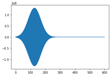
pulse = G.gaussianPulse(time,energy=energy,amplitude=pars['field_amplitude'],fwhm=fwhm)
time unit: fs - energy unit: eV
period of the oscillations 2.757111798154881 fs
width of the pulse 42.466090014400955 fs
fwhm of the pulse 100 fs
[10]:
plt.plot(time,pulse)
[10]:
[<matplotlib.lines.Line2D at 0x7fee646c5130>]
[11]:
Omega = lambda t : G.gaussianPulse(t,energy=energy,amplitude=pars['Omega0_abs'],fwhm=fwhm,envelope_only=True,verbose=False)
[12]:
uprime0 = np.array([0.,0.,1.])
[13]:
delta = 30 # in meV
delta_fsm1 = 1e-3*delta/h_red # in fs^-1
[16]:
uprime = TLS.solveBlochEq(uprime0,time,Omega,mu12=dipole,delta=delta_fsm1)
[17]:
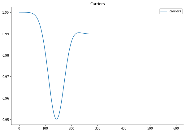
plt.figure(figsize=(10,7))
plt.title('Carriers')
plt.plot(time,(1+uprime[2])/2,label='carriers')
plt.legend()
plt.show()
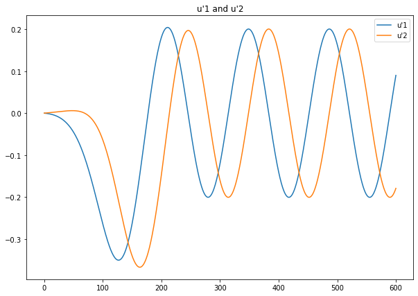
plt.figure(figsize=(10,7))
plt.plot(time,uprime[0],label="u'1")
plt.plot(time,uprime[1],label="u'2")
plt.title("u'1 and u'2")
plt.legend()
[17]:
<matplotlib.legend.Legend at 0x7fee5c558b50>
[18]:
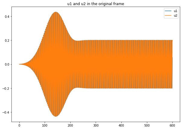
u = TLS.convertToRotatingFrame(omega,time,uprime,invert=True)
[19]:
plt.figure(figsize=(10,7))
plt.plot(time,u[0],label='u1')
plt.plot(time,u[1],label='u2')
plt.title('u1 and u2 in the original frame')
plt.legend()
[19]:
<matplotlib.legend.Legend at 0x7fee5c4e9550>
Global response of many \(k\)-points to a gaussian pulse. Emergence of the FID.
We consider the global response of the system with a large samplings of \(k\)-points.
To each point there is an associated detuning and we assume a uniform distribution in a given energy range.
[20]:
import random as rand
[21]:
numk = 1000
delta_range = 40 # meV
deltas = [0.] # the first kpoint has zero detuning
for i in range(numk-1):
    deltas.append(delta_range*(rand.random()-0.5))
We set the properties of the system and of the pulse. Here we assume for symplicity that all k the points have the same value of the transition dipole
[22]:
T = 4000 #fs
tstep = int(4e3)
dipole = 1 +1j # the weight of the real and imaginary part can be changed
time = np.linspace(0,T,tstep)

fwhm =  100 # fs
energy = 1.5 # pulse energy in eV
omega = energy/(C.Planck_reduced_ev_ps*1e3) # angular frequency of the pulse

h_red = C.Planck_reduced_ev_ps*1e3 # hbar in eV*fs
We choose a field that realizes the \(\pi/2\) condition (for the points with zero detuning)
[23]:
theta1= 0.5*np.pi # set the area of the pulse
pars1 = TLS.pulseParametersFromTheta(dipole,theta1,fwhm=fwhm)
pars1
time unit: fs
the width parameter of the pulse is 42.466090014400955 fs
Rabi coupling (fs^-1): (0.010434524642511517+0.010434524642511517j)
Rabi coupling (module) (fs^-1): 0.014756646266356059
field amplitude (V/m): 129788828.49284193
field intensity (kW/cm^2) : 4471405.517491325
[23]:
{'Omega0': (0.010434524642511517+0.010434524642511517j),
 'Omega0_abs': 0.014756646266356059,
 'field_amplitude': 129788828.49284193,
 'intensity': 4471405.517491325}
[24]:
Omega = lambda t : G.gaussianPulse(t,energy=energy,amplitude=pars1['Omega0_abs'],fwhm=fwhm,envelope_only=True,verbose=False)
[28]:
#plt.plot(time,Omega(time))
[35]:
uprime0 = np.array([0.,0.,1.]) # set the system in the GS before the pulse
[36]:
uprime = np.zeros([3,len(time),numk])
for k in range(numk):
    delta_fsm1 = 1e-3*deltas[k]/h_red
    uprime[:,:,k] = TLS.solveBlochEq(uprime0,time,Omega,mu12=dipole,delta=delta_fsm1)
uprime_global = np.mean(uprime,axis=2)
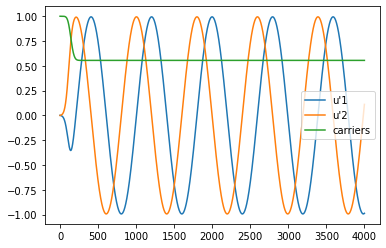
[37]:
k = 3
plt.plot(time,uprime[0,:,k],label="u'1")
plt.plot(time,uprime[1,:,k],label="u'2")
plt.plot(time,0.5*(1+uprime[2,:,k]),label="carriers")
plt.legend()
[37]:
<matplotlib.legend.Legend at 0x7fee5c391ac0>
[38]:
plt.figure(figsize=(10,7))
plt.plot(time,uprime_global[0],label="u'1")
plt.plot(time,uprime_global[1],label="u'2")
plt.plot(time,0.5*(1-uprime_global[2]),label="carriers")
plt.legend()
[38]:
<matplotlib.legend.Legend at 0x7fee5c558b80>
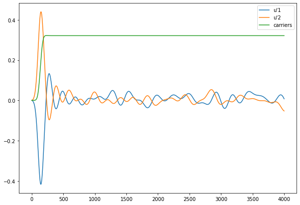
The emergence of the Free Induction Decay (FID) mechanism is clearly visible.
Echo mechanism in the \(\pi/2\) - \(\pi\) configuration
We add a second \(\pi\) pulse to realize the echo mechanism.
[40]:
theta2= np.pi # set the area of the pulse
pars2 = TLS.pulseParametersFromTheta(dipole,theta2,fwhm=fwhm)
pars2
time unit: fs
the width parameter of the pulse is 42.466090014400955 fs
Rabi coupling (fs^-1): (0.020869049285023034+0.020869049285023034j)
Rabi coupling (module) (fs^-1): 0.029513292532712117
field amplitude (V/m): 259577656.98568386
field intensity (kW/cm^2) : 17885622.0699653
[40]:
{'Omega0': (0.020869049285023034+0.020869049285023034j),
 'Omega0_abs': 0.029513292532712117,
 'field_amplitude': 259577656.98568386,
 'intensity': 17885622.0699653}
[41]:
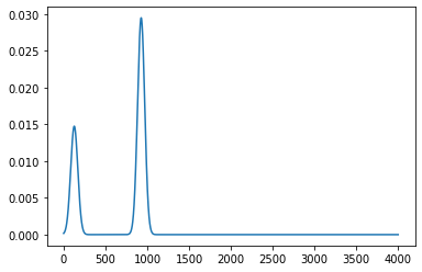
Omega = lambda t : G.doubleGaussianPulse(t,energy=energy,amplitude1=pars1['Omega0_abs'],amplitude2=pars2['Omega0_abs'],
                    fwhm1=fwhm,fwhm2=fwhm,t_start2=800,envelope_only=True,verbose=False)
[42]:
plt.plot(time,Omega(time))
[42]:
[<matplotlib.lines.Line2D at 0x7fee5c1fa850>]
[43]:
uprime0 = np.array([0.,0.,1.]) # set the system in the GS before the pulse
[45]:
uprime = np.zeros([3,len(time),numk])
for k in range(numk):
    delta_fsm1 = 1e-3*deltas[k]/h_red
    uprime[:,:,k] = TLS.solveBlochEq(uprime0,time,Omega,mu12=dipole,delta=delta_fsm1)
uprime_global = np.mean(uprime,axis=2)
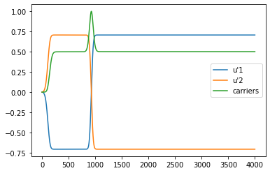
[46]:
k = 0
plt.plot(time,uprime[0,:,k],label="u'1")
plt.plot(time,uprime[1,:,k],label="u'2")
plt.plot(time,0.5*(1-uprime[2,:,k]),label="carriers")
plt.legend()
[46]:
<matplotlib.legend.Legend at 0x7fee5c1b07f0>
[48]:
plt.figure(figsize=(10,7))
plt.plot(time,uprime_global[0],label="u'1")
plt.plot(time,uprime_global[1],label="u'2")
plt.plot(time,0.5*(1-uprime_global[2]),label="carriers")
plt.legend()
[48]:
<matplotlib.legend.Legend at 0x7fee5c122bb0>
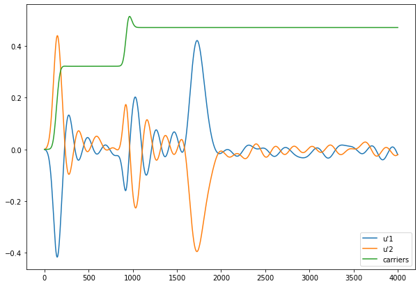
The echo signal emerges.
[ ]: