[1]:
# useful to autoreload the module without restarting the kernel
%load_ext autoreload
%autoreload 2
[2]:
from mppi import InputFiles as I, Calculators as C, Utilities as U, Parsers as P
from mppi.Calculators import Tools
import matplotlib.pyplot as plt
## use ipyml for interactive plots
%matplotlib inline
import numpy as np
import os
[3]:
omp = 1
mpi = 4
Tutorial of the YamboParser class
This tutorial describes the usage of the YamboParser class. The parser contains instances of several classes, namely : * the YamboOutputParser that deals with the o- file(s) produced by a yambo computation * the YamboDipolesParser that parse the dipoles database created by Yambo * the YamboDftParser that extract lattice and electronic information (ad the dft level) from the ns.db1 database written by Yambo in the SAVE folder
The class is designed to deal with the output of the run method of YamboCalculator.
Here we present a first example by performing a gw calculation:
[5]:
rr = C.RunRules(mpi=mpi,omp_num_threads=omp)
code = C.YamboCalculator(rr)
Initialize a Yambo calculator with scheduler direct
[6]:
input_dir = 'QeCalculator_test/outdir_nscf/bands_8.save'
[7]:
run_dir = 'YamboCalculator_test'
Tools.init_yambo_dir(yambo_dir=run_dir,input_dir=input_dir,overwrite_if_found=False)
SAVE folder YamboCalculator_test/SAVE already present. No operations performed.
[8]:
inp = I.YamboInput(args='yambo -d -k hartee -g n -p p -V qp',folder=run_dir)
inp.set_kRange(1,2)
#inp
[37]:
results = code.run(input = inp, run_dir = run_dir, name='qp_test1')
results
Skip the run of qp_test1
[37]:
{'output': {'qp': 'YamboCalculator_test/qp_test1/o-qp_test1.qp'},
 'report': 'YamboCalculator_test/qp_test1/r-qp_test1_HF_and_locXC_gw0_dyson_em1d_ppa_el_el_corr',
 'dft': 'YamboCalculator_test/SAVE/ns.db1',
 'QP': 'YamboCalculator_test/qp_test1/ndb.QP',
 'HF_and_locXC': 'YamboCalculator_test/qp_test1/ndb.HF_and_locXC',
 'dipoles': 'YamboCalculator_test/qp_test1/ndb.dipoles',
 'pp': 'YamboCalculator_test/qp_test1/ndb.pp'}
The calculator contain the references to the o- files and database with the output data. The parser extract the data from the files, as follows
[38]:
P.YamboParser?
Init signature: P.YamboParser(results, verbose=False, extendOut=True)
Docstring:
Class that perform the parsing starting from the results :py:class:`dict` built
by the :class:`YamboCalculator` class. In the actual implementation of the class the
parser is able to deal with the o- files, the dipoles database, the ``ndb.RT_G_PAR``
and the ``ns.db1`` database written in the SAVE folder.

Args:
    results (:py:class:`dict`): The dictionary of the results built by the
        :class:`YamboCalculator` class
    verbose (:py:class:`boolean`) : Determine the amount of information provided on terminal
    extendOut (:py:class:`boolean`) : Determine which dictionary is used as reference for the
                    names of the variables in the :class:`YamboOutputParser`

Attributes:
    data (:class:`YamboOutputParser`) : contains the instance of the :class:`YamboOutputParser`
        class that manage the parsing of the ``o-* files``
    dipoles (:class:`YamboDipolesParser`) : contains the instance of the :class:`YamboDipolesParser`
        class that manages the parsing of the ``dipoles`` database
    dft (:class:`YamboDftParser`) : contains the instance of the :class:`YamboDftParser` that
        manages the parsing of the ``ns.db1`` database
    qp (:class:`YamboQPParser`) : contains the instance of the :class:`YamboQPParser` that
        manages the parsing of the ``ndb.QP`` database
    RTCarriers (:class:`YamboRTCarriersParser`) : contains the instance of the
        :class:`YamboRTCarriersParser` that manages the parsing of the `ndb.RT_carriers`
        database
    RTGreen (:class:`YamboRTGlesserParser`) : contains the instance of the
        :class:`YamboRTGlesserParser` that manages the parsing of the `ndb.RT_G_PAR`
        database
Init docstring: Initialize the data member of the class.
File:           ~/Applications/MPPI/mppi/Parsers/YamboParser.py
Type:           type
Subclasses:
Note that the extendOut option has to chosen in agreement with the one the input, otherwise the parser atribute the name of the variables of the o- files in an erroneous way
[39]:
data = P.YamboParser(results,extendOut=False,verbose=True)
Parse file YamboCalculator_test/qp_test1/o-qp_test1.qp
Parse file : YamboCalculator_test/SAVE/ns.db1
Parse file : YamboCalculator_test/qp_test1/ndb.QP
Parse file : YamboCalculator_test/qp_test1/ndb.dipoles
Spin dipoles not found in the ndb.dipoles
Some information on the parsed data can be obtained using the get_info method of the class
[40]:
data.get_info()
YamboOutputParser variables structure
suffix qp with dict_keys(['kpoint', 'band', 'E0', 'EmE0', 'sce0'])

YamboDipolesParser variables structure
dip_ir shape (32, 4, 4, 3, 2)
dip_p shape (32, 4, 4, 3, 2)
dip_v shape (32, 4, 4, 3, 2)
dip_spin shape (1,)

YamboDftParser variables structure
number of k points 32
number of bands 8
spin degeneration 1

YamboQPParser variables structure
QP_table shape (16, 3)
QP_kpts shape (32, 3)
QP_E shape (16, 2)
QP_Eo shape (16,)
QP_Z shape (16, 2)
Data are encapsulated in the attributes of the class, for instance
[23]:
data.data
[23]:
{'qp': {'kpoint': array([1., 1., 1., 1., 1., 1., 1., 1., 2., 2., 2., 2., 2., 2., 2., 2.]),
  'band': array([1., 2., 3., 4., 5., 6., 7., 8., 1., 2., 3., 4., 5., 6., 7., 8.]),
  'E0': array([-1.189685e+01, -1.216440e-06,  0.000000e+00,  0.000000e+00,
          2.565152e+00,  2.565152e+00,  2.565152e+00,  3.146653e+00,
         -1.153855e+01, -2.375836e+00, -4.453420e-01, -4.453410e-01,
          2.294498e+00,  3.205499e+00,  3.205499e+00,  5.284825e+00]),
  'EmE0': array([-1.564291,  0.722413,  0.741914,  0.741673,  1.86755 ,  1.867259,
          1.829724,  2.395583, -1.427122,  0.369035,  0.648066,  0.670303,
          1.853613,  1.981288,  1.955341,  2.673125]),
  'sce0': array([ 4.57619 ,  2.008809,  2.031459,  2.031144, -2.003587, -2.003874,
         -2.046769, -1.926959,  4.600586,  2.457894,  2.028683,  2.054817,
         -1.999774, -2.067204, -2.096922, -1.932993])}}
[13]:
data.dft
[13]:
<mppi.Parsers.YamboDftParser.YamboDftParser at 0x7f4707cc38e0>
[14]:
data.dipoles
[14]:
<mppi.Parsers.YamboDipolesParser.YamboDipolesParser at 0x7f4707cc3250>
In what follows we describe the features of the various classes using dedicated examples
A YamboParser object can be also instanciated directly using the name of the folders that contain the o-* files and the databases, for instance
[52]:
outputPath = 'YamboCalculator_test/qp_test1'
[53]:
data2 = P.YamboParser.from_path(run_dir=run_dir,outputPath=outputPath,verbose=True,extendOut=False)
Parse file YamboCalculator_test/qp_test1/o-qp_test1.qp
Parse file : YamboCalculator_test/SAVE/ns.db1
Parse file : YamboCalculator_test/qp_test1/ndb.QP
Parse file : YamboCalculator_test/qp_test1/ndb.dipoles
Spin dipoles not found in the ndb.dipoles
[54]:
data2.get_info()
YamboOutputParser variables structure
suffix qp with dict_keys(['kpoint', 'band', 'E0', 'EmE0', 'sce0'])

YamboDipolesParser variables structure
dip_ir shape (32, 4, 4, 3, 2)
dip_p shape (32, 4, 4, 3, 2)
dip_v shape (32, 4, 4, 3, 2)
dip_spin shape (1,)

YamboDftParser variables structure
number of k points 32
number of bands 8
spin degeneration 1

YamboQPParser variables structure
QP_table shape (16, 3)
QP_kpts shape (32, 3)
QP_E shape (16, 2)
QP_Eo shape (16,)
QP_Z shape (16, 2)
Analysis of the YamboOutputParser class
The class is designed to deal with the list of o- files produced by Yambo We present some example:
[25]:
qp_output = {'qp' : 'YamboParser_test/qp_results/o-qp_test1.qp'}
[26]:
qp_output_extendOut = {'qp' : 'YamboCalculator_test/qp_test_ExtendOut/o-qp_test_ExtendOut.qp'}
[37]:
rt_output = {'carriers':'YamboParser_test/rt_results/o-NETime_1000-dephase_0.01-freq_1.55-pol_circular.carriers',
             'spin_magnetization':'YamboParser_test/rt_results/o-NETime_1000-dephase_0.01-freq_1.55-pol_circular.spin_magnetization',
             'external_field':'YamboParser_test/rt_results/o-NETime_1000-dephase_0.01-freq_1.55-pol_circular.external_field',
             'polarization':'YamboParser_test/rt_results/o-NETime_1000-dephase_0.01-freq_1.55-pol_circular.polarization'}
When the list of files is passed to the parser the extendOut option used to run the computation has to be provided, otherwise the parser could perform a wrong assignement of the names of the variables.
[27]:
P.YamboOutputParser?
Init signature: P.YamboOutputParser(output, verbose=True, extendOut=True)
Docstring:
Class that performs the parsing of a Yambo o- file(s). The class ineriths from :py:class:`dict`
and the instance of the class is a dictionary with the data. The keys correspond to the extension
of the parsed files.

Args:
    output (:py:class:`list`): Dictionary with the structure of the output of :py:meth:`get_output_files`
        of the `YamboCalculator` module.
    verbose (:py:class:`boolean`) : Determine the amount of information provided on terminal
    extendOut (:py:class:`boolean`) : Determine which dictionary is used as reference for the
                    names of the variables
Init docstring: Initialize the data member of the class.
File:           ~/Applications/MPPI/mppi/Parsers/YamboOutputParser.py
Type:           type
Subclasses:
[29]:
results = P.YamboOutputParser(output=qp_output,extendOut=False)
Parse file YamboParser_test/qp_results/o-qp_test1.qp
results is a dictionary with the structure
[30]:
results
[30]:
{'qp': {'kpoint': array([1., 1., 1., 1., 1., 1., 1., 1., 2., 2., 2., 2., 2., 2., 2., 2.]),
  'band': array([1., 2., 3., 4., 5., 6., 7., 8., 1., 2., 3., 4., 5., 6., 7., 8.]),
  'E0': array([-1.190291e+01, -1.176000e-05, -1.176000e-05,  0.000000e+00,
          2.551225e+00,  2.551230e+00,  2.551230e+00,  3.152071e+00,
         -1.110872e+01, -3.914389e+00, -7.552550e-01, -7.552460e-01,
          1.962407e+00,  3.490390e+00,  3.490396e+00,  6.757975e+00]),
  'EmE0': array([-1.50691 ,  0.7861  ,  0.7914  ,  0.7771  ,  1.884047,  1.907533,
          1.906476,  2.349819, -1.21027 ,  0.216875,  0.676644,  0.653277,
          1.799721,  2.065016,  2.084261,  2.726886]),
  'sce0': array([ 4.48108 ,  2.194   ,  2.201   ,  2.184061, -2.137494, -2.110904,
         -2.112035, -2.203245,  4.52994 ,  2.934759,  2.263484,  2.236098,
         -2.186759, -2.20382 , -2.182057, -2.267519])}}
For several usages it can be useful to access to the results with the object.attribute sintax. In this case it is possible to use the AttributeDict class the perform this conversion
[33]:
obj = U.AttributeDict(**results)
and we can access as
[34]:
obj.qp.E0
[34]:
array([-1.190291e+01, -1.176000e-05, -1.176000e-05,  0.000000e+00,
        2.551225e+00,  2.551230e+00,  2.551230e+00,  3.152071e+00,
       -1.110872e+01, -3.914389e+00, -7.552550e-01, -7.552460e-01,
        1.962407e+00,  3.490390e+00,  3.490396e+00,  6.757975e+00])
Test of a parsing with extendOut = True
[35]:
results = P.YamboOutputParser(output=qp_output_extendOut,extendOut=True)
Parse file YamboCalculator_test/qp_test_ExtendOut/o-qp_test_ExtendOut.qp
now all the variables are available, for instance
[36]:
results['qp']['z_Re']
[36]:
array([0.724502, 0.846966, 0.847311, 0.847307, 0.839802, 0.839785,
       0.839137, 0.853679, 0.719236, 0.823056, 0.842047, 0.842398,
       0.844161, 0.839568, 0.839091, 0.850125])
Let’s see a further example by parsing the typical files of a real-time computation
[38]:
results = P.YamboOutputParser(rt_output)
Parse file YamboParser_test/rt_results/o-NETime_1000-dephase_0.01-freq_1.55-pol_circular.carriers
Parse file YamboParser_test/rt_results/o-NETime_1000-dephase_0.01-freq_1.55-pol_circular.spin_magnetization
Parse file YamboParser_test/rt_results/o-NETime_1000-dephase_0.01-freq_1.55-pol_circular.external_field
Parse file YamboParser_test/rt_results/o-NETime_1000-dephase_0.01-freq_1.55-pol_circular.polarization
In this case we have several files, so the dictionary has more than one key
[39]:
results.keys()
[39]:
dict_keys(['carriers', 'spin_magnetization', 'external_field', 'polarization'])
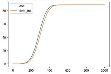
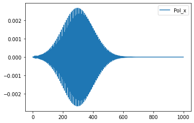
We can easily perform some plots
[40]:
time = results['carriers']['time']
elec = results['carriers']['dne']
field_int = results['external_field']['Intensity']
pol = results['polarization']['Pol_x']

ratio = max(field_int)/max(elec)

plt.plot(time,ratio*elec,label='dne')
plt.plot(time,field_int,label='field_int')
plt.legend()
plt.show()

plt.plot(time,pol,label='Pol_x')
plt.legend()
[40]:
<matplotlib.legend.Legend at 0x7f9cad0ef5b0>
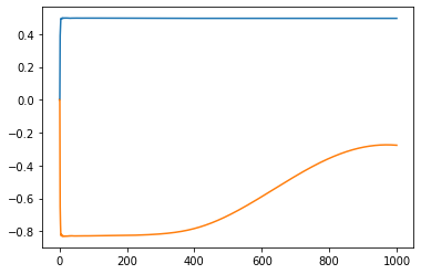
Again we can access to the results using the attribute syntax. For instance if we are intersted to the spin_magnetization part of the resutls we can set
[41]:
spin_results = U.AttributeDict(**results['spin_magnetization'])
[42]:
plt.plot(spin_results.time,spin_results.Mc_z)
plt.plot(spin_results.time,spin_results.Mv_z)
[42]:
[<matplotlib.lines.Line2D at 0x7f9cacfaedf0>]
YamboOutputParser for a ypp computation
We test the functionality of the Parser to deal with the output of a ypp -s b computation for plotting the bands structure along a path
[43]:
bands_output = {'bands_interpolated':'YamboCalculator_test/bands_test1/o-bands_test1.bands_interpolated'}
[44]:
results = P.YamboOutputParser(bands_output)
Parse file YamboCalculator_test/bands_test1/o-bands_test1.bands_interpolated
For instance
[45]:
results['bands_interpolated']['col0'] # kpath
[45]:
array([0.        , 0.04593836, 0.09187671, 0.13781506, 0.18375342,
       0.22969177, 0.27563013, 0.32156848, 0.36750684, 0.41344519,
       0.45938355, 0.5053219 , 0.55126025, 0.59719861, 0.64313696,
       0.68907532, 0.73501367, 0.78095203, 0.82689038, 0.87282874,
       0.91876709, 0.96470544, 1.0106438 , 1.0565822 , 1.1017687 ,
       1.1469552 , 1.19214171, 1.23732823, 1.28251474, 1.32770126,
       1.37288778, 1.4180743 , 1.46326081, 1.50844733, 1.55363385,
       1.59882037, 1.64400689, 1.6891934 , 1.73437992, 1.77956644,
       1.82475296, 1.86993948, 1.91512599, 1.96031251, 2.005499  ,
       2.05068555, 2.09587206, 2.14105858, 2.1862451 , 2.2314316 ,
       2.2766181 , 2.3235426 , 2.3704671 , 2.41739152, 2.46431598,
       2.51124044, 2.5581649 , 2.60508936, 2.65201382, 2.69893828,
       2.74586274, 2.79278721, 2.83971167, 2.88663613, 2.93210418,
       2.97757224, 3.0230403 , 3.06850835, 3.11397641, 3.15944447,
       3.20491252, 3.25038058, 3.29584864, 3.34131669, 3.38678475,
       3.43225281, 3.47772086, 3.52318892, 3.56865697, 3.61412503,
       3.65959309, 3.70506114, 3.7505292 , 3.79599726, 3.84146531,
       3.88693337, 3.93240143, 3.97786948, 4.02333754, 4.0688056 ,
       4.11427365, 4.1597417 , 4.2052098 , 4.2506778 ])
[46]:
results['bands_interpolated']['col1'] # energies of the first band included in the computation
[46]:
array([-1.35540660e-06, -1.35540660e-06, -2.37583629e+00, -2.37583629e+00,
       -2.37583629e+00, -2.37583629e+00, -5.30497690e+00, -5.30497690e+00,
       -5.30497690e+00, -5.30497690e+00, -4.42422173e+00, -4.42422173e+00,
       -2.05464056e+00, -2.05464056e+00, -5.30497690e+00, -5.30497690e+00,
       -5.30497690e+00, -5.30497690e+00, -2.37583629e+00, -2.37583629e+00,
       -2.37583629e+00, -2.37583629e+00, -1.35540660e-06, -1.35540660e-06,
       -1.35540660e-06, -1.35540660e-06, -2.05464056e+00, -2.05464056e+00,
       -2.05464056e+00, -2.05464056e+00, -5.00667257e+00, -5.00667257e+00,
       -5.00667257e+00, -5.00667257e+00, -5.00667257e+00, -7.78724511e+00,
       -7.78724511e+00, -7.78724511e+00, -7.78724511e+00, -5.00667257e+00,
       -5.00667257e+00, -5.00667257e+00, -5.00667257e+00, -5.00667257e+00,
       -1.35540660e-06, -2.05464056e+00, -2.05464056e+00, -2.05464056e+00,
       -1.35540660e-06, -1.35540660e-06, -1.35540660e-06, -1.35540660e-06,
       -1.35540660e-06, -2.05464056e+00, -2.05464056e+00, -2.05464056e+00,
       -2.05464056e+00, -5.00667257e+00, -5.00667257e+00, -5.00667257e+00,
       -5.00667257e+00, -7.78724511e+00, -7.78724511e+00, -7.78724511e+00,
       -7.78724511e+00, -7.78724511e+00, -7.67094267e+00, -7.67094267e+00,
       -6.74725642e+00, -5.63143757e+00, -5.63143757e+00, -6.74725642e+00,
       -6.74725642e+00, -6.74725642e+00, -6.74725642e+00, -6.74725567e+00,
       -7.67094267e+00, -7.67094267e+00, -6.74725567e+00, -7.67094267e+00,
       -7.67094267e+00, -6.54702153e+00, -5.63143688e+00, -5.63143688e+00,
       -5.63143688e+00, -5.63143688e+00, -3.71240251e+00, -4.42422154e+00,
       -2.05464056e+00, -2.05464056e+00, -2.05464056e+00, -1.35540660e-06,
       -1.35540660e-06, -1.35540660e-06])
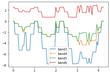
The parser cannot determine the names of the columns because the number of colums depend on the number of bands considered. The meaning of the columns can be identified by knowing the input used to perform the post processing.
[47]:
r = results['bands_interpolated']
kpath = r['col0']
band3 = r['col1']
band4 = r['col2']
band5 = r['col3']
band6 = r['col4']
[48]:
plt.plot(kpath,band3,label='band3')
plt.plot(kpath,band4,label='band4')
plt.plot(kpath,band5,label='band5')
plt.plot(kpath,band6,label='band6')
plt.legend()
[48]:
<matplotlib.legend.Legend at 0x7f9cacf895e0>
Analysis of the YamboDipolesParser class
To analyze the YamboDipolesParser we build the dipoles using Yambo. We start from a nscf computation on GaAs on a regular grid with 12 bands (8 full and 4 empties, since the bands are spin splitted)
[ ]:
source_dir = 'Pw_bands/gaas_nscf_so.save'
save_dir = Tools.make_p2y(source_dir,overwrite_if_found=False)
[54]:
run_dir = 'YamboParser_test/DipolesParser'
Tools.init_yambo_run_dir(save_dir,run_dir,overwrite_if_found=False,make_link=True)
Create folder YamboParser_test/DipolesParser
Executing command: cd Pw_bands/gaas_nscf_so.save; p2y
Create a symlink of /home/marco/Applications/MPPI/sphinx_source/tutorials/Pw_bands/gaas_nscf_so.save/SAVE in YamboParser_test/DipolesParser
Executing command: cd YamboParser_test/DipolesParser;OMP_NUM_THREADS=1 mpirun -np 1 yambo
[55]:
inp = I.YamboInput(args='yambo -dipoles -V all',folder=run_dir)
inp['variables']['DipComputed'] = 'R P V Spin'
inp['arguments'].append("DipBandsALL")
inp
[55]:
{'args': 'yambo -dipoles -V all',
 'folder': 'YamboParser_test/DipolesParser',
 'filename': 'yambo.in',
 'arguments': ['DipBandsALL'],
 'variables': {'StdoHash': [40.0, ''],
  'Nelectro': [8.0, ''],
  'ElecTemp': [0.0, 'eV'],
  'BoseTemp': [-1.0, 'eV'],
  'OccTresh': [1e-05, ''],
  'NLogCPUs': [0.0, ''],
  'MEM_tresh': [51200.0, 'Kb'],
  'DIP_Threads': [0.0, ''],
  'DipoleEtresh': [1e-05, 'eV'],
  'DBsIOoff': 'none',
  'DBsFRAGpm': 'none',
  'PAR_def_mode': 'balanced',
  'DipComputed': 'R P V Spin',
  'DipBands': [[1, 12], '']}}
Note that the options DipBandsALL enables the computation of the dipoles elements among all the bands, and not only in for the full-empty couples
[56]:
code.run(input=inp,run_dir=run_dir,name='dipoles',mpi=1,skip=False)
run command: mpirun -np 1 yambo -F dipoles.in -J dipoles -C dipoles
computation dipoles is running...
computation dipoles ended

        There are no o-* files.
        Maybe you have performed a ypp computation or wait_end_run and/or
        the dry_run option are active.
        Otherwise a possible error has occured during the computation

Run performed in 06s
[56]:
{'output': {},
 'report': 'YamboParser_test/DipolesParser/dipoles/r-dipoles_dipoles',
 'dft': 'YamboParser_test/DipolesParser/SAVE/ns.db1',
 'dipoles': 'YamboParser_test/DipolesParser/dipoles/ndb.dipoles'}
Once that the computation is over, and the database is built by Yambo we parse it
[57]:
dipole_file = os.path.join(run_dir,'dipoles/ndb.dipoles')
[58]:
dipoles = P.YamboDipolesParser(dipole_file)
Parse file : YamboParser_test/DipolesParser/dipoles/ndb.dipoles
[59]:
dipoles.get_info()
YamboDipolesParser variables structure
dip_ir shape (16, 12, 12, 3, 2)
dip_p shape (16, 12, 12, 3, 2)
dip_v shape (16, 12, 12, 3, 2)
dip_spin shape (16, 12, 12, 3, 2)
We consider the r dipole (x component) and look for the values of the valence->conduction elements
[63]:
k = 0
vb = 7
cb = 8
print(dipoles.r_dipole(k,vb,cb,0))
print(dipoles.r_dipole(k,cb,vb,0))
[[[ 0.00000000e+00+0.00000000e+00j -7.32989130e+00-1.04414460e+00j
   -2.67618113e-04-2.73337086e-02j -8.31398256e-01-8.24659863e-01j
    1.54225410e-02+5.53155198e-01j -8.47292442e-03-3.52913430e-02j
    3.94122962e-02+4.51266933e-01j -3.50684921e-02-4.23464784e-02j
   -3.27529949e-03+3.62501186e-03j  3.12675546e-02-8.78397798e-02j
   -6.91983853e-03-5.34757557e-03j  5.07940800e-03-9.23038442e-02j]
  [-7.32989130e+00+1.04414460e+00j  0.00000000e+00+0.00000000e+00j
    8.01318921e-01+8.54408462e-01j -3.56489315e-02-9.21653706e-03j
   -9.18567469e-03-1.86620892e-02j  5.51941446e-01+1.59714051e-03j
   -8.44179368e-03-1.80563835e-02j -4.53646536e-01+2.62720464e-02j
   -3.27381201e-02-8.40906364e-02j  2.53831680e-03-5.56781058e-03j
    2.48079709e-02-9.19902074e-02j  5.51535117e-03+1.76623507e-03j]
  [-2.67618113e-04+2.73337086e-02j  8.01318921e-01-8.54408462e-01j
    0.00000000e+00+0.00000000e+00j  1.89030428e+00+4.66548965e-01j
    5.79517535e-02+7.19914584e-02j  2.97413490e-01+5.37567659e-01j
    3.39576600e-02+1.71525456e-02j  1.13901180e+00-2.80942908e-02j
   -1.35458846e-01+8.48610027e-02j -5.79681904e-03-1.26648203e-02j
   -8.71556302e-02-1.00831534e-01j -5.21431367e-03+1.90947218e-02j]
  [-8.31398256e-01+8.24659863e-01j -3.56489315e-02+9.21653706e-03j
    1.89030428e+00-4.66548965e-01j  0.00000000e+00+0.00000000e+00j
    5.45636211e-01-3.35822521e-01j  1.14411805e-02-7.20224684e-02j
    2.58112611e-02+1.15460258e+00j -1.03327761e-02+2.34740261e-03j
   -9.08485260e-03+1.39249252e-02j  1.57530187e-01+1.64761717e-02j
   -9.18993867e-03-6.50085470e-03j  1.11691402e-01+7.31907914e-02j]
  [ 1.54225410e-02-5.53155198e-01j -9.18567469e-03+1.86620892e-02j
    5.79517535e-02-7.19914584e-02j  5.45636211e-01+3.35822521e-01j
    0.00000000e+00+0.00000000e+00j  2.11427743e-01-9.56134044e-01j
    1.62831255e+00-7.55540099e-01j  6.61581637e-02+1.10979076e-01j
   -9.25205611e-02+4.45597370e-02j  1.38243035e-01+2.87229424e-01j
    4.08191950e-02-2.36504566e-04j  2.30604964e-01+2.95389137e-01j]
  [-8.47292442e-03+3.52913430e-02j  5.51941446e-01-1.59714051e-03j
    2.97413490e-01-5.37567659e-01j  1.14411805e-02+7.20224684e-02j
    2.11427743e-01+9.56134044e-01j  0.00000000e+00+0.00000000e+00j
   -5.85802578e-02-1.12608495e-01j -1.63776512e+00+7.00740450e-01j
   -1.39602536e-01+3.03461916e-01j -5.13598540e-02+6.83745581e-02j
   -3.35693039e-01+1.78584191e-01j -7.62539820e-03-1.13538619e-02j]
  [ 3.94122962e-02-4.51266933e-01j -8.44179368e-03+1.80563835e-02j
    3.39576600e-02-1.71525456e-02j  2.58112611e-02-1.15460258e+00j
    1.62831255e+00+7.55540099e-01j -5.85802578e-02+1.12608495e-01j
    0.00000000e+00+0.00000000e+00j -2.28599993e+01-4.96581405e+01j
   -1.40120452e-03-3.13814570e-02j  3.07801000e+00-1.74927227e+00j
   -8.07164003e-03-1.42328602e-02j -8.70404117e-01+5.57876659e-01j]
  [-3.50684921e-02+4.23464784e-02j -4.53646536e-01-2.62720464e-02j
    1.13901180e+00+2.80942908e-02j -1.03327761e-02-2.34740261e-03j
    6.61581637e-02-1.10979076e-01j -1.63776512e+00-7.00740450e-01j
   -2.28599993e+01+4.96581405e+01j  0.00000000e+00+0.00000000e+00j
   -3.38338401e+00-1.12316434e+00j -8.75460474e-03-8.31172632e-04j
    4.99613685e-01+9.46940754e-01j  8.01958247e-03-4.09287053e-02j]
  [-3.27529949e-03-3.62501186e-03j -3.27381201e-02+8.40906364e-02j
   -1.35458846e-01-8.48610027e-02j -9.08485260e-03-1.39249252e-02j
   -9.25205611e-02-4.45597370e-02j -1.39602536e-01-3.03461916e-01j
   -1.40120452e-03+3.13814570e-02j -3.38338401e+00+1.12316434e+00j
    0.00000000e+00+0.00000000e+00j -1.38856218e+00-5.58888916e+00j
   -2.31086113e+00+1.17762304e+00j -1.41328812e-01+1.49001606e-01j]
  [ 3.12675546e-02+8.78397798e-02j  2.53831680e-03+5.56781058e-03j
   -5.79681904e-03+1.26648203e-02j  1.57530187e-01-1.64761717e-02j
    1.38243035e-01-2.87229424e-01j -5.13598540e-02-6.83745581e-02j
    3.07801000e+00+1.74927227e+00j -8.75460474e-03+8.31172632e-04j
   -1.38856218e+00+5.58888916e+00j  0.00000000e+00+0.00000000e+00j
    2.52960030e-02-1.81659493e-01j -7.61363207e-01+2.53330306e+00j]
  [-6.91983853e-03+5.34757557e-03j  2.48079709e-02+9.19902074e-02j
   -8.71556302e-02+1.00831534e-01j -9.18993867e-03+6.50085470e-03j
    4.08191950e-02+2.36504566e-04j -3.35693039e-01-1.78584191e-01j
   -8.07164003e-03+1.42328602e-02j  4.99613685e-01-9.46940754e-01j
   -2.31086113e+00-1.17762304e+00j  2.52960030e-02+1.81659493e-01j
    0.00000000e+00+0.00000000e+00j -4.97362491e+00+1.64461368e+01j]
  [ 5.07940800e-03+9.23038442e-02j  5.51535117e-03-1.76623507e-03j
   -5.21431367e-03-1.90947218e-02j  1.11691402e-01-7.31907914e-02j
    2.30604964e-01-2.95389137e-01j -7.62539820e-03+1.13538619e-02j
   -8.70404117e-01-5.57876659e-01j  8.01958247e-03+4.09287053e-02j
   -1.41328812e-01-1.49001606e-01j -7.61363207e-01-2.53330306e+00j
   -4.97362491e+00-1.64461368e+01j  0.00000000e+00+0.00000000e+00j]]]
[]
we observe that inverting the order of the bands changes sign to the imaginary part of the matrix element, as expected.
Analysis of the YamboDftParser class
This database collects information about the lattice and electronic properties of the system.
The information codified in this database are usually equivalent to the ones in the QuantumESPRESSO data-file-schema.xml and the YamboDftParser shares many common functions with the PwParser.
To perform a comparison we consider the example of bulk WSe2, that has a exaghonal symmetry (ibrav=4 in pw input) with layered structure in the \(z\) direction. We consider a 12x12x3 \(k\)-sampling with 100 bands and we compare the data-file-schema.xml and the ns.db1 database.
[30]:
xml = 'YamboParser_test/dftParsers_results/WSe2_12x12x3_100bands/data-file-schema.xml'
nsdb = 'YamboParser_test/dftParsers_results/WSe2_12x12x3_100bands/ns.db1'
[31]:
pw_data = P.PwParser(xml)
yambo_data = P.YamboDftParser(nsdb)
Parse file : YamboParser_test/dftParsers_results/WSe2_12x12x3_100bands/data-file-schema.xml
Parse file : YamboParser_test/dftParsers_results/WSe2_12x12x3_100bands/ns.db1
[32]:
print(yambo_data.alat)
print(yambo_data.lattice)
print(yambo_data.nbands)
print(yambo_data.nbands_full)
print(yambo_data.spin_degen)
print(len(yambo_data.syms))
yambo_data.syms[1]
[ 6.198302   5.3678865 24.483292 ]
[[ 6.198302   0.         0.       ]
 [-3.099151   5.3678865  0.       ]
 [ 0.         0.        24.483292 ]]
100
52
1
12
[32]:
array([[ 1.0000001,  0.       ,  0.       ],
       [ 0.       , -1.       ,  0.       ],
       [ 0.       ,  0.       , -1.0000001]], dtype=float32)
[33]:
print(pw_data.alat)
print(pw_data.lattice)
6.198301719262
[[ 6.19830172  0.          0.        ]
 [-3.09915086  5.36788675  0.        ]
 [ 0.          0.         24.48329179]]
Note that Yambo uses a vector alat variable. For this reason if we compare the expression of the lattice vector expressed in units of alat and the ones of the reciprocal axis vector expressed in units of 2:math:`pi`/alat they have different components. This can be confirmed by looking in the log and in r_setup file in the folder ``YamboParser_test/dftParsers_results/WSe2_12x12x3_100bands``.
[34]:
pw_data.get_lattice(rescale=True)
[34]:
array([[ 1.       ,  0.       ,  0.       ],
       [-0.5      ,  0.8660254,  0.       ],
       [ 0.       ,  0.       ,  3.95     ]])
[35]:
yambo_data.get_lattice(rescale=True)
[35]:
array([[ 1.       ,  0.       ,  0.       ],
       [-0.5      ,  0.8660254,  0.       ],
       [ 0.       ,  0.       ,  3.9499998]], dtype=float32)
Note that the get_lattice method of yambo_data rescale the lattice vectors w.r.t the first component of the vector alat parameter of yambo, so the result is equivalent to the one of the pw_data class.
Due to the same approach also the reciprocal lattice are consistent in the two classes
[36]:
pw_data.get_reciprocal_lattice(rescale=True)
[36]:
array([[ 1.        ,  0.57735027, -0.        ],
       [ 0.        ,  1.15470054,  0.        ],
       [ 0.        , -0.        ,  0.25316456]])
[37]:
yambo_data.get_reciprocal_lattice(rescale=True)
[37]:
array([[ 1.        ,  0.5773503 , -0.        ],
       [ 0.        ,  1.1547006 ,  0.        ],
       [ 0.        , -0.        ,  0.25316456]], dtype=float32)
We also compare the expressions of the k-points
[38]:
pw_data.kpoints[0:20]
[38]:
array([[ 0.        ,  0.        ,  0.        ],
       [ 0.        ,  0.        ,  0.08438819],
       [ 0.        ,  0.09622504,  0.        ],
       [ 0.        ,  0.09622504,  0.08438819],
       [ 0.        ,  0.19245009,  0.        ],
       [ 0.        ,  0.19245009,  0.08438819],
       [ 0.        ,  0.28867513,  0.        ],
       [ 0.        ,  0.28867513,  0.08438819],
       [ 0.        ,  0.38490018,  0.        ],
       [ 0.        ,  0.38490018,  0.08438819],
       [ 0.        ,  0.48112522,  0.        ],
       [ 0.        ,  0.48112522,  0.08438819],
       [ 0.        , -0.57735027,  0.        ],
       [ 0.        , -0.57735027,  0.08438819],
       [ 0.08333333,  0.14433757,  0.        ],
       [ 0.08333333,  0.14433757,  0.08438819],
       [ 0.08333333,  0.24056261,  0.        ],
       [ 0.08333333,  0.24056261,  0.08438819],
       [ 0.08333333,  0.33678766,  0.        ],
       [ 0.08333333,  0.33678766,  0.08438819]])
[39]:
yambo_data.kpoints[0:20]
[39]:
array([[ 0.        ,  0.        ,  0.        ],
       [ 0.        ,  0.        ,  0.33333334],
       [ 0.        ,  0.08333333,  0.        ],
       [ 0.        ,  0.08333333,  0.33333334],
       [ 0.        ,  0.16666666,  0.        ],
       [ 0.        ,  0.16666666,  0.33333334],
       [ 0.        ,  0.24999999,  0.        ],
       [ 0.        ,  0.24999999,  0.33333334],
       [ 0.        ,  0.3333333 ,  0.        ],
       [ 0.        ,  0.3333333 ,  0.33333334],
       [ 0.        ,  0.41666666,  0.        ],
       [ 0.        ,  0.41666666,  0.33333334],
       [ 0.        , -0.49999997,  0.        ],
       [ 0.        , -0.49999997,  0.33333334],
       [ 0.08333334,  0.12499999,  0.        ],
       [ 0.08333334,  0.12499999,  0.33333334],
       [ 0.08333334,  0.20833333,  0.        ],
       [ 0.08333334,  0.20833333,  0.33333334],
       [ 0.08333334,  0.29166666,  0.        ],
       [ 0.08333334,  0.29166666,  0.33333334]], dtype=float32)
Which are different because they represent the cart. coord. in units 2pi/alat and again yambo uses a vector alat.
[40]:
yambo_data.get_kpoints(use_scalar_alat=True)[0:20]
[40]:
array([[ 0.        ,  0.        ,  0.        ],
       [ 0.        ,  0.        ,  0.08438819],
       [ 0.        ,  0.09622505,  0.        ],
       [ 0.        ,  0.09622505,  0.08438819],
       [ 0.        ,  0.19245009,  0.        ],
       [ 0.        ,  0.19245009,  0.08438819],
       [ 0.        ,  0.28867513,  0.        ],
       [ 0.        ,  0.28867513,  0.08438819],
       [ 0.        ,  0.38490018,  0.        ],
       [ 0.        ,  0.38490018,  0.08438819],
       [ 0.        ,  0.48112527,  0.        ],
       [ 0.        ,  0.48112527,  0.08438819],
       [ 0.        , -0.57735026,  0.        ],
       [ 0.        , -0.57735026,  0.08438819],
       [ 0.08333334,  0.14433756,  0.        ],
       [ 0.08333334,  0.14433756,  0.08438819],
       [ 0.08333334,  0.24056263,  0.        ],
       [ 0.08333334,  0.24056263,  0.08438819],
       [ 0.08333334,  0.33678767,  0.        ],
       [ 0.08333334,  0.33678767,  0.08438819]], dtype=float32)
In this way the components are equal to the ones of the pw_data class.
The class contain also methods to compute the lattice volume
[27]:
yambo_data.eval_lattice_volume(rescale=False)
[27]:
814.6027
[28]:
pw_data.eval_lattice_volume(rescale=False)
[28]:
814.6027389471978
[25]:
yambo_data.eval_reciprocal_lattice_volume(rescale=True)
[25]:
0.29232928
[26]:
pw_data.eval_reciprocal_lattice_volume(rescale=True)
[26]:
0.2923292502226171
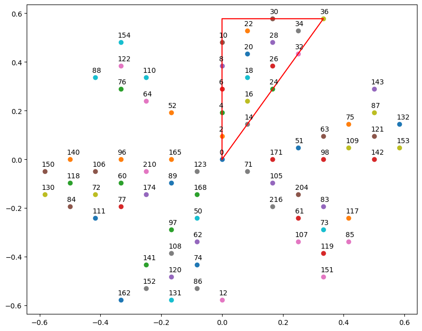
Lastly, we show the kpoints distribution after a Fixsymm procedure. We use the same WSe2 calculation but we load the ndb obtained after the Fixsymm.
[12]:
dft_ndb = 'YamboParser_test/rt_results/ns.db1'
fixsymm_data = P.YamboDftParser(dft_ndb)
Parse file : YamboParser_test/rt_results/ns.db1
[13]:
kpoints = fixsymm_data.get_kpoints(use_scalar_alat=True)
[14]:
# in cartesian coordinates
Gamma = np.array([0.,0.,0.])
K = np.array([1/3.,1/np.sqrt(3.),0])
M = np.array([0.,1/np.sqrt(3.),0])
[15]:
numk = kpoints.shape[0]
numk
[15]:
222
[19]:
fig, ax = plt.subplots(figsize=(10, 8))

for ind in range(numk): # limit to 50 for the non expanded grid
    if kpoints[ind,2] == 0.: # project on the xy plane
        plt.scatter(kpoints[ind,0],kpoints[ind,1])
        plt.text(kpoints[ind,0]-0.01,kpoints[ind,1]+0.02,ind)
IBZ = [Gamma[0:2],K[0:2], M[0:2],Gamma[0:2]]
plt.plot(*np.column_stack(IBZ),color='red')
[19]:
[<matplotlib.lines.Line2D at 0x7fb098acc700>]
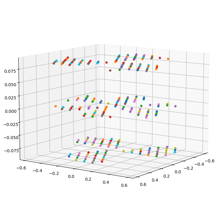
[17]:
fig = plt.figure(figsize=(9, 9))
ax = fig.add_subplot(projection='3d')
ax.view_init(10, 35)
for ind in range(numk):
    ax.scatter3D(kpoints[ind,0],kpoints[ind,1],kpoints[ind,2])
plt.show()
Analysis of the YamboQPParser class
This database collects information about the quasi-particle correction
[59]:
qp_ndb = 'YamboCalculator_test/qp_test1/ndb.QP'
qp_data = P.YamboQPParser(qp_ndb)
Parse file : YamboCalculator_test/qp_test1/ndb.QP
[8, 32, 16, 0, 0, 24]
[61]:
from netCDF4 import Dataset
[62]:
d = Dataset(qp_ndb)
[65]:
d['PARS'][:]
[65]:
masked_array(data=[ 8., 32., 16.,  0.,  0., 24.],
             mask=False,
       fill_value=1e+20,
            dtype=float32)
[66]:
d
[66]:
<class 'netCDF4._netCDF4.Dataset'>
root group (NETCDF4 data model, file format HDF5):
    dimensions(sizes): D_0000000001(1), D_0000000003(3), D_0000000002(2), D_0000000100(100), D_0000000006(6), QP_desc_size(24), QP_string_len(100), D_0000000016(16), D_0000000032(32)
    variables(dimensions): float32 QP_DB_kind(D_0000000001), float32 HEAD_VERSION(D_0000000003), float32 HEAD_REVISION(D_0000000001), float32 SERIAL_NUMBER(D_0000000001), float32 SPIN_VARS(D_0000000002), float32 HEAD_D_LATT(D_0000000003), |S1 CUTOFF(D_0000000001, D_0000000100), float32 TEMPERATURES(D_0000000002), |S1 G_energies_xc_KIND(D_0000000001, D_0000000100), |S1 G_wavefunctions_xc_KIND(D_0000000001, D_0000000100), |S1 Xp_energies_xc_KIND(D_0000000001, D_0000000100), |S1 Xp_wavefunctions_xc_KIND(D_0000000001, D_0000000100), float32 PARS(D_0000000006), int32 QP_N_DESCRIPTORS(D_0000000001), int32 QP_DESCRIPTORS_SIZES(QP_desc_size), |S1 QP_DESCRIPTORS_NAMES(QP_desc_size, QP_string_len), |S1 QP_DESCRIPTORS_KINDS(QP_desc_size, QP_string_len), |S1 QP_DESCRIPTORS_TERMS(QP_desc_size, QP_string_len), |S1 QP_GW_solver(D_0000000001, D_0000000100), |S1 QP_GW_approximation(D_0000000001, D_0000000100), float32 QP_PPA_imaginary_Energy(D_0000000001), int32 QP_GW_SC_iterations(D_0000000001), int32 QP_dS_dw_steps(D_0000000001), float32 QP_dS_dw_step(D_0000000001), int32 QP_X_Gs(D_0000000001), int32 QP_X_bands(D_0000000002), float32 QP_X_poles(D_0000000001), float32 QP_X_e_h_E_range(D_0000000002), |S1 QP_X_Hxc_Kernel(D_0000000001, D_0000000100), int8 QP_X_BZ_energy_Double_Grid(D_0000000001), int32 QP_Sc_G_bands(D_0000000002), float32 QP_Sc_G_damping(D_0000000001), int8 QP_Sc_bands_terminator(D_0000000001), int32 QP_Sx_RL_components(D_0000000001), |S1 QP_EMPTY_STR_Nr18(D_0000000001, D_0000000100), int32 QP_QP_@_state_1_K_range(D_0000000002), int32 QP_QP_@_state_1_b_range(D_0000000002), |S1 QP_GF_energies_kind(D_0000000001, D_0000000100), |S1 QP_GF_WFs_kind(D_0000000001, D_0000000100), |S1 QP_Xs_energies_kind(D_0000000001, D_0000000100), |S1 QP_Xs_WFs_kind(D_0000000001, D_0000000100), float32 QP_table(D_0000000003, D_0000000016), float32 QP_kpts(D_0000000003, D_0000000032), float32 QP_E(D_0000000016, D_0000000002), float32 QP_Eo(D_0000000016), float32 QP_Z(D_0000000016, D_0000000002)
    groups:
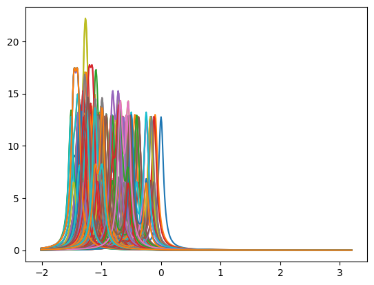
Analysis of the YamboRTCarriersParser class
This database collects information about the time, energy and \(k\)-points distribution of the real-time carriers.
We consider the test case of a RT simulation performed on bulk WSe2 on a 12x12x3 k-sampling (with a Fixsymm procedure due to the linear external field in the \(x\) direction). The ns.db1 associated built by the Fixsymm is included in the folder
[23]:
rt_ndb = 'YamboParser_test/rt_results/ndb.RT_carriers'
dft_ndb = 'YamboParser_test/rt_results/ns.db1'
[24]:
rt_data = P.YamboRTCarriersParser(rt_ndb)
dft_data = P.YamboDftParser(dft_ndb)
Parse file : YamboParser_test/rt_results/ndb.RT_carriers
Parse file : YamboParser_test/rt_results/ns.db1
[25]:
rt_data.get_info()
YamboRTCarriersParser variables structure
Bands used and number of k-points [ 49  54 222]
kpoints shape (222, 3)
E_bare shape (1332,)
f_bare shape (1332,)
delta_E shape (16, 1332)
delta_f (16, 1332)
[58]:
d = rt_data.build_f_bare_dos(eta=0.05,dE=0.01)
[59]:
len(d.dos)
[59]:
222
[60]:
d.plot(plt,legend=False)